2022-03-19

数学建模实验 III 平面图形几何变换

Author: `sandyzikun`

简单介绍其基于OpenCV的实现.

Problem Description

平面图形的几何变换:

使用齐次坐标实现平面图形的旋转, 缩放, 以及平移变换.
任意实例化一个2维平面向量, 要求给出变换公式及程式;
求出 $ 3 \times 3 $ 矩阵, 对应于先乘以 $ 3 $ 的倍乘变换, 然后逆时针旋转 $ \frac{\pi}2 $, 最后对图形的每个点的坐标加上 $ (-2, 6) $ 做平移, 并作实例化;
利用matlab函数imwarp(), 实现图像的旋转和缩放, 并作实例化(任取一幅图像);

Problem Analysis

使用OpenCV¹进行实现.

OpenCV是一个跨语言计算机视觉模块, 其拥有把图像读取为三轴张量并存储为数组, 以及对图像数组进行变换的方法.
对于其Python实现, 其形式上为使用C++编写的本体上加载Python接口.

Basic Methods

.imread(filename[, flags]) -> retval: Loads an image from a file.
根据filename所示路径读取图像文件, 存储为(三轴)张量的方法, 默认以BGR格式进行存储;
.imshow(winname, mat) -> None: Displays an image in the specified window.
创建标题为winname的窗体, 显示变量mat所存储的张量对应的图像.
需要注意与matplotlib.pyplot的.imshow相区分;
- .imshow(X, cmap=None, norm=None, aspect=None, interpolation=None, alpha=None, vmin=None, vmax=None, origin=None, extent=None, shape=None, filternorm=1, filterrad=4.0, imlim=None, resample=None, url=None, hold=None, data=None, **kwargs): Display an image on the axes.
  顾名思义matplotlib.pyplot的.imshow是在画布的坐标轴上显示图像, 但这属于matplotlib的内容, 在此不进行赘述;
- 但后面我们会使用matplotlib.pyplot的.imshow;
.waitKey([, delay]) -> retval: Waits for a pressed key.
通过OpenCV呼出显示图像窗体后使之正常停留在屏幕中, 等待下一动作的方法 ~~, 不使用这个方法的话经常会使窗体卡死~~;
destroyAllWindows() -> None: Destroys all of the HighGUI windows.
用于在程式结束前检查并关闭所有通过OpenCV呼出而未关闭的窗体的函数;

`OpenCV` Method `.resize`

.resize是对图像进行缩放的方法, 查看其说明

Python

>>> cv2.resize?
resize(src, dsize[, dst[, fx[, fy[, interpolation]]]]) -> dst
.   @brief Resizes an image.
...

可知使用.resize至少需要传入待变换的图像src与变换后的目标尺寸dsize, 可以用参数interpolation指定大小变换的插值方法, 例如

Python

>>> cv2.resize(
...     img_arr,
...     (img_width // 2, img_height // 2),
...     interpolation=cv2.INTER_CUBIC # Using Cubic Interpolation / 使用二次曲线插值
...     )

便返回对img_arr缩小至原本的0.5的图像, 并且使用二次曲线插值,

Python

>>> cv2.resize(
...     img_arr,
...     (img_width * 2, img_height * 2),
...     interpolation=cv2.INTER_LINEAR # Using Linear Interpolation / 使用线性插值
...     )

便返回对img_arr放大至原本2倍的图像, 并用线性插值.

`OpenCV` Method `.warpAffine`

.warpAffine是对图像进行仿射变换的方法, 查看其说明

Python

>>> cv2.warpAffine?
warpAffine(src, M, dsize[, dst[, flags[, borderMode[, borderValue]]]]) -> dst
.   @brief Applies an affine transformation to an image.
.
.   The function warpAffine transforms the source image using the specified matrix:
.
.   \f[\texttt{dst} (x,y) =  \texttt{src} ( \texttt{M} _{11} x +  \texttt{M} _{12} y +  \texttt{M} _{13}, \texttt{M} _{21} x +  \texttt{M} _{22} y +  \texttt{M} _{23})\f]

可知其操作便是根据式

$\begin{align*} \texttt{dst} (x,y) = \texttt{src} ( & \texttt{M} _{11} x + \texttt{M} _{12} y + \texttt{M} _{13}, \\ & \texttt{M} _{21} x + \texttt{M} _{22} y + \texttt{M} _{23} ) \end{align*}$

从图像变量src生成dst的内容.

Images in Linear Algebra

在讲述平面图形的几何变换之前, 我们需要先明确几个概念.

齐次坐标 (Homogeneous Coordinates) ³: m维射影空间 (Projective Space) ⁴的点对应的等价类 (Equivalence Class) ⁵中每个(m+1)元组⁶.
例如二维坐标点Q(x, y)的齐次坐标便为(hx, hy, h), 取h=1时便有规格化的齐次坐标(x, y, 1);
(图像的)空间变换 (Spacial Transformation): 图像在计算机中(经过采样和量化)存储为一个以像素颜色为元素的矩阵, 虽然各个像素形式上为这个矩阵中的元素, 但其格式也有多种, 包括但不限于RGB(包括BGR等其实都一样的), HSV, CMYK等, 此时对所有的点进行统一的变换即达到对整幅图像进行变换的效果;

Modeling

然后我们来考虑几种平面图像的几何变换.

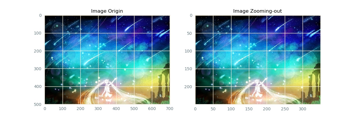
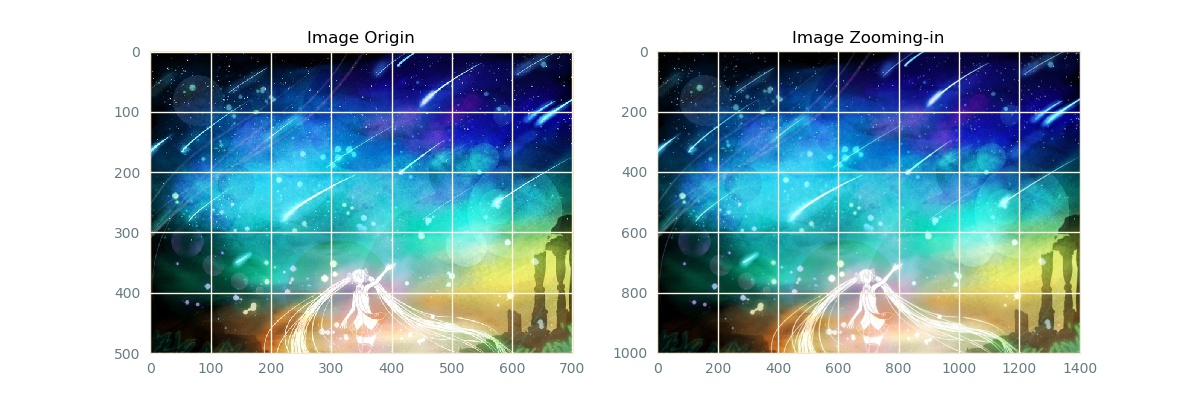
Image Resizing

图像缩放变换 $ (x, y) \mapsto (s x, t y) $, 可以简单使用矩阵乘法实现

$\begin{bmatrix} s & 0 & 0 \\ 0 & t & 0 \\ 0 & 0 & 1 \\ \end{bmatrix} \begin{pmatrix} x \\ y \\ 1 \\ \end{pmatrix} = \begin{pmatrix} s x \\ t y \\ 1 \\ \end{pmatrix}$

然后使用.resize即可.

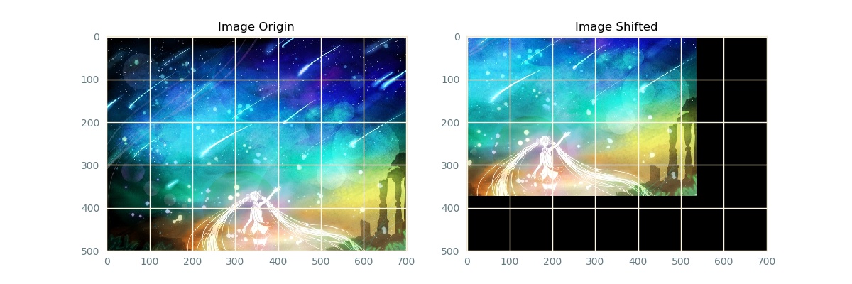
Image Shifting

图像平移变换 $ (x, y) \mapsto (x + a, y + b) $, 齐次坐标写作 $ (x, y, 1) \mapsto (x + a, y + b, 1) $, 可以简单使用矩阵乘法进行实现

$\begin{bmatrix} 1 & 0 & a \\ 0 & 1 & b \\ 0 & 0 & 1 \\ \end{bmatrix} \begin{pmatrix} x \\ y \\ 1 \\ \end{pmatrix} = \begin{pmatrix} x + a \\ y + b \\ 1 \\ \end{pmatrix}$

而在OpenCV中我们.warpAffine对图像进行变换时, 对其中的参数M传入变换矩阵前两行的 $ 2 \times 3 $ 矩阵即可.

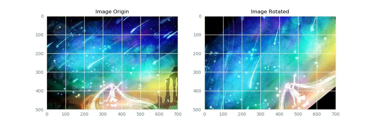
Image Rotation

图像旋转变换 $ (x, y) \mapsto (x \cos \theta - y \sin \theta , x \sin \theta + y \cos \theta) $, 可以使用矩阵乘法实现

$\begin{bmatrix} \cos \theta & - \sin \theta & 0 \\ \sin \theta & \cos \theta & 0 \\ 0 & 0 & 1 \\ \end{bmatrix} \begin{pmatrix} x \\ y \\ 1 \\ \end{pmatrix} \\ = \begin{pmatrix} x \cos \theta - y \sin \theta \\ x \sin \theta + y \cos \theta \\ 1 \\ \end{pmatrix}$

在OpenCV中需要传入图像旋转的中心点center, 角度angle, 以及缩放尺寸scale, 用.getRotationMatrix2D计算旋转变换的矩阵, 然后作为参数M传入.warpAffine即可.

Affine Transformation

参考这些文章².

Processing Image with `OpenCV`

在此简要演示OpenCV完整读取与处理图像的用法.
首先声明调用NumPy, matplotlib.pyplot及OpenCV等模块

Python

import numpy as np
from matplotlib import pyplot as plt
plt.style.use("solarized-light") # 我自己做的一个matplotlib配色方案, 这个不是它自带的, 该行可以不写
import cv2

我们以如下所示的图片⁷对上述方法及任务进行演示:

我们先通过.imread读取图像并把其对应的张量存入变量arr_icsk,

Python

1	>>> arr_icsk = cv2.imread("./ichisaki-01.jpeg")

查看该变量

Python

>>> arr_icsk
array([[[255, 255, 255],
        [255, 255, 255],
        [255, 255, 255],
        ...,
        [255, 255, 255],
        [255, 255, 255],
        [255, 255, 255]],

       [[255, 255, 255],
        [255, 255, 255],
        [255, 255, 255],
        ...,
        [255, 255, 255],
        [255, 255, 255],
        [255, 255, 255]],

       ...,

       [[255, 255, 255],
        [255, 255, 255],
        [255, 255, 255],
        ...,
        [255, 255, 255],
        [255, 255, 255],
        [255, 255, 255]]], dtype=uint8)

可见这其实被直接转化为了一个NumPy的.ndarray对象, 因此我们可以调用属于它固有的成员或方法

Python

>>> arr_icsk.ndim # 查看张量轴数, 由于这是一个彩色非透明图像, 所以会存储为三轴张量, 因此其轴数便为3
3

>>> arr_icsk.shape # 查看张量尺寸
(1440, 1727, 3)

>>> arr_icsk[ : , : , 0 ].mean() # 查看蓝色channel的平均亮度值, 由于OpenCV存储图像的格式为BGR而非RGB, 因此蓝色channel对应索引为0
230.49256860001287

>>> arr_icsk[ : , : , 1 ].mean() # 对应索引为1的绿色channel的平均亮度值
241.52439040082353

>>> arr_icsk[ : , : , 2 ].mean() # 对应索引为2的红色channel的平均亮度值
254.97663176349482

我们所取用图片的尺寸过大, 因此我们用.resize把它的宽度和高度缩小到原本的1/3.9

Python

>>> height, width, num_channels = arr_icsk.shape

>>> arr_icsk = cv2.resize(
...     arr_icsk,
...     (round(width / 3.9), round(height / 3.9)),
...     interpolation = cv2.INTER_CUBIC
...     )

需要注意的是图像存入ndarray的格式是(height, width, num_channels), 但传入的参数却是(width, height).
然后我们调用.imshow显示图像

Python

1	>>> cv2.imshow("Image Display", arr_icsk)

但是得到的却是一个灰色的窗体, 而且容易卡死, 这时候我们调用.waitKey让其等待动作

Python

1 2	>>> cv2.waitKey() -1

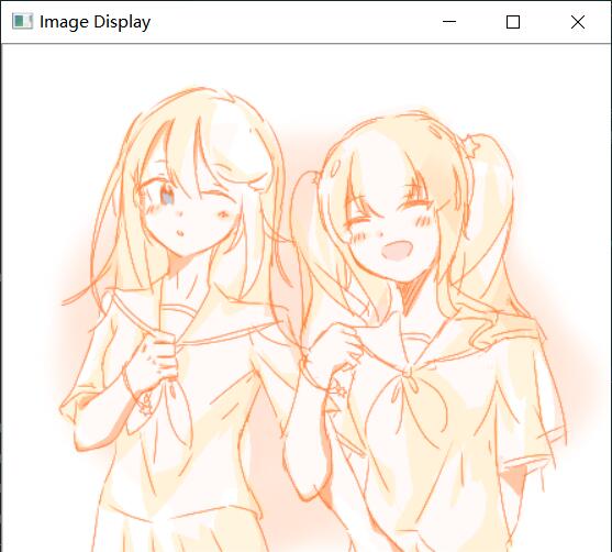
便能正常显示.
然后关闭窗口即可结束.waitKey的等待, 此时这个函数本身会返回-1.
为了保险起见, 我们可以调用.destroyAllWindows关闭呼出的所有窗体.

Python

1	>>> cv2.destroyAllWindows()

以上是使用OpenCV的.imread进行图像的显示, 但是我们可以使用我们熟悉的matplotlib相关功能进行类似的操作, 但这里要注意OpenCV存储与读取的是BGR格式, matplotlib读取的是RGB格式, 所以我们要先对张量的通道顺序进行调整

Python

1	>>> arr_icsk = arr_icsk[ : , : , : : (-1) ]

然后再调用matplotlib.pyplot的.imshow

Python

>>> plt.imshow(arr_icsk)
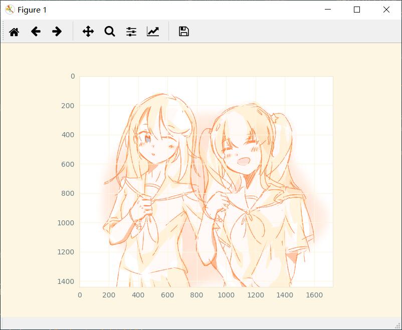
<matplotlib.image.AxesImage at 0x20b6a828e80>

>>> plt.show() # 显示图像

得到如上所示的可视化结果, matplotlib.pyplot还会标注坐标轴, 此外还可以利用子图, 标题等功能对可视化的结果加入其他内容

Python

>>> plt.title("Image ICHISAKI Display via plt.imshow()") # 设置标题
Text(0.5,1,'Image ICHISAKI Display via plt.imshow()')

>>> plt.xlabel("Axis of width") # 设置x轴信息
Text(0.5,0,'Axis of width')

>>> plt.ylabel("Axis of height") # 设置y轴信息
Text(0,0.5,'Axis of height')

>>> plt.imshow(arr_icsk)
<matplotlib.image.AxesImage at 0x20b6b34fd68>

>>> plt.show()

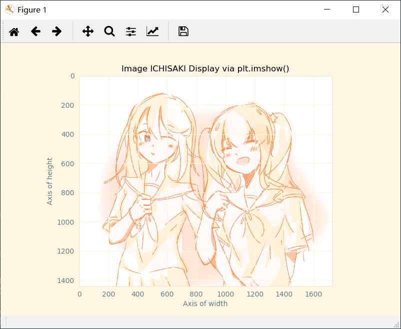
这样便能显示带有标题和轴标注的图像.

Solving

现在我们考虑题目给出的任务.

T1: 对于矢量(3, 9), 进行如下操作便分别有对应结果:

旋转 $ \frac{\pi}4 $, 得到矢量 $ (3 \cos \frac{\pi}4 - 9 \sin \frac{\pi}4 , 3 \sin \frac{\pi}4 + 9 \cos \frac{\pi}4) = (- 3 \sqrt{2}, 6 \sqrt{2}) $;
放大2倍, 得到矢量(6, 18);
平移(5, 1)得到矢量(8, 10);

T2: $ 当 \psi = \frac{\pi}2 时, \sin \psi = 1, \cos \psi = 0. 此时有 $

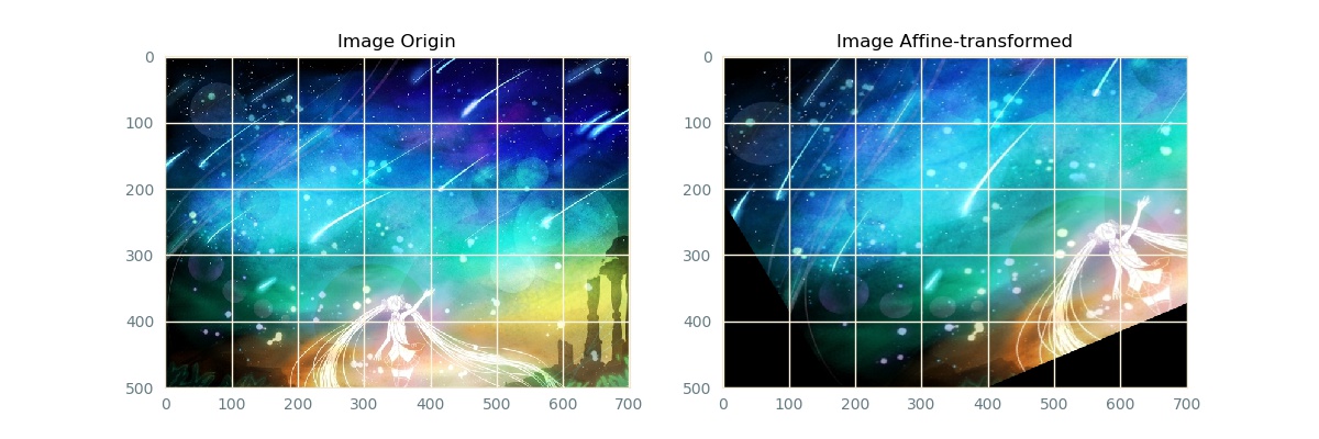
$\begin{align*} \begin{pmatrix} x \\ y \\ 1 \\ \end{pmatrix} \xrightarrow[]{缩放} & \begin{bmatrix} 3 & 0 & 0 \\ 0 & 3 & 0 \\ 0 & 0 & 1 \\ \end{bmatrix} \begin{pmatrix} x \\ y \\ 1 \\ \end{pmatrix} \\ \xrightarrow[]{旋转} & \begin{bmatrix} 0 & -1 & 0 \\ 1 & 0 & 0 \\ 0 & 0 & 1 \\ \end{bmatrix} \begin{bmatrix} 3 & 0 & 0 \\ 0 & 3 & 0 \\ 0 & 0 & 1 \\ \end{bmatrix} \begin{pmatrix} x \\ y \\ 1 \\ \end{pmatrix} \\ \xrightarrow[]{平移} & \begin{bmatrix} 1 & 0 & -2 \\ 0 & 1 & 6 \\ 0 & 0 & 1 \\ \end{bmatrix} \begin{bmatrix} 0 & -1 & 0 \\ 1 & 0 & 0 \\ 0 & 0 & 1 \\ \end{bmatrix} \begin{bmatrix} 3 & 0 & 0 \\ 0 & 3 & 0 \\ 0 & 0 & 1 \\ \end{bmatrix} \begin{pmatrix} x \\ y \\ 1 \\ \end{pmatrix} \\ = & \begin{bmatrix} 0 & -3 & -2 \\ 3 & 0 & 6 \\ 0 & 0 & 1 \\ \end{bmatrix} \begin{pmatrix} x \\ y \\ 1 \\ \end{pmatrix} \end{align*}$

T3: 对于如下图像¹¹

我们将进行缩放, 平移, 旋转, 以及仿射变换. 完整程式如下

Python

#!/usr/bin/env Python
# -*- coding: utf-8 -*-

"""
@author: 陈 子坤 (GitHub@sandyzikun)
@time: 2022-03-19 18:39
"""

import numpy as np, cv2
from matplotlib import pyplot as plt
plt.style.use("solarized-light")

class Constants(object):
    PATH_IMAGE = "./meteor.jpeg"

if __name__ == "__main__":
    plt.rcParams["figure.figsize"] = (12, 4)
    #plt.rcParams["figure.facecolor"] = "#fdf6e3"
    img_arr = cv2.imread(Constants.PATH_IMAGE)
    img_height, img_width, _ = img_arr.shape
    # Image Zooming-out / 图像缩小
    """
    cv2.imshow(
        "Image Zooming-out",
        cv2.resize(
            img_arr,
            (img_width // 2, img_height // 2),
            interpolation=cv2.INTER_CUBIC # Using Cubic Interpolation / 使用二次曲线插值
            )
        )
    cv2.waitKey()
    """
    plt.subplot(121)
    plt.title("Image Origin")
    plt.imshow(img_arr[ : , : , : : (-1) ])
    plt.subplot(122)
    plt.title("Image Zooming-out")
    plt.imshow(
        cv2.resize(
            img_arr,
            (img_width // 2, img_height // 2),
            interpolation=cv2.INTER_CUBIC # Using Cubic Interpolation / 使用二次曲线插值
            )[ : , : , : : (-1) ]
        )
    plt.savefig("./fig-01.jpeg")
    plt.show()
    plt.clf()
    # Image Zooming-in / 图像放大
    plt.subplot(121)
    plt.title("Image Origin")
    plt.imshow(img_arr[ : , : , : : (-1) ])
    plt.subplot(122)
    plt.title("Image Zooming-in")
    plt.imshow(
        cv2.resize(
            img_arr,
            (img_width * 2, img_height * 2),
            interpolation=cv2.INTER_LINEAR # Using Linear Interpolation / 使用线性插值
            )[ : , : , : : (-1) ]
        )
    plt.savefig("./fig-02.jpeg")
    plt.show()
    plt.clf()
    # Image Shifting / 图像平移
    plt.subplot(121)
    plt.title("Image Origin")
    plt.imshow(img_arr[ : , : , : : (-1) ])
    plt.subplot(122)
    plt.title("Image Shifted")
    plt.imshow(
        cv2.warpAffine(
            img_arr,
            np.float32([ # Transformation (Shifting) Matrix (shape: 2x3)
                [ 1 , 0 , -164 ],
                [ 0 , 1 , -128 ],
                ]),
            (img_width, img_height)
            )[ : , : , : : (-1) ]
        )
    plt.savefig("./fig-03.jpeg")
    plt.show()
    plt.clf()
    # Image Rotation / 图像旋转
    plt.subplot(121)
    plt.title("Image Origin")
    plt.imshow(img_arr[ : , : , : : (-1) ])
    plt.subplot(122)
    plt.title("Image Rotated")
    plt.imshow(
        cv2.warpAffine(
            img_arr,
            cv2.getRotationMatrix2D(
                (round(img_width / 2), round(img_height / 2)),
                39,
                1.28
                ),
            (img_width, img_height)
            )[ : , : , : : (-1) ]
        )
    plt.savefig("./fig-04.jpeg")
    plt.show()
    plt.clf()
    # Affine Transformation / 仿射变换
    plt.subplot(121)
    plt.title("Image Origin")
    plt.imshow(img_arr[ : , : , : : (-1) ])
    plt.subplot(122)
    plt.title("Image Affine-transformed")
    plt.imshow(
        cv2.warpAffine(
            img_arr,
            cv2.getAffineTransform(
                np.float32([
                    [  50 ,  50 ],
                    [ 200 ,  50 ],
                    [  50 , 200 ],
                    ]),
                np.float32([
                    [  10 , 100 ],
                    [ 200 ,  20 ],
                    [ 100 , 250 ],
                    ])
                ),
            (img_width, img_height)
            )[ : , : , : : (-1) ]
        )
    plt.savefig("./fig-05.jpeg")
    plt.show()
    plt.clf()

运行结果如下

Image Zooming-out (图像缩小)
Image Zooming-in (图像缩大)
Image Shifting (图像平移)
Image Rotation (图像旋转)
Affine Transformation (仿射变换)

Extra

事实上图像的相关操作在matlab的Image Processing Toolbox工具箱¹²中有相关实现, 主要依靠imwarp方法¹³并把缩放, 平移, 旋转等操作全部以仿射变换的形式完成. 但由于在octave的image¹⁴包中并无相关实现¹⁵, 故在此不再过多赘述.

于此介绍keras.preprocessing.image中的.apply_transform()方法. 我们先调用

Python

1	>>> keras.preprocessing.image.apply_transform?

来查看一下它的说明, 得到以下信息

Python

1	keras.preprocessing.image.apply_transform(x, transform_matrix, channel_axis=0, fill_mode='nearest', cval=0.0)

Apply the image transformation specified by a matrix.

Arguments
- x: 2D numpy array, single image.
- transform_matrix: Numpy array specifying the geometric transformation.
- channel_axis: Index of axis for channels in the input tensor.
- fill_mode: Points outside the boundaries of the input are filled according to the given mode (one of {'constant', 'nearest', 'reflect', 'wrap'}).
- cval: Value used for points outside the boundaries of the input if mode='constant'.
Returns
The transformed version of the input.

由此我们可以知道, 这个函数中通过参数x传入待变换的图像张量, 限制为RGB类格式.
由于图像张量通常为三轴, 因此需要在参数channel_aixs中指出排列不同通道的轴, 由于OpenCV和Keras调用的PIL都是在最后一个轴排列通道, 故此处我们必须向其指出channel_axis=2, 如若是Theano则需要指定channel_axis=0.
图像对坐标变换后常有出现某位置原本有像素点但变换后像素点消失的情况, 对于这一方面的问题我们需要在fill_mode中指定填充缺失位置的填充方案, 在此介绍常用的两种:

constant: 用灰度色彩的常量进行填充, 需要通过参数cval指定填充用的灰度值, 即空出的部分皆会被涂满cval所示亮度的灰度;
nearest: 默认的填充方案, 会选取距离待填充点最近的已填充点的颜色进行填充;

我们现在来使用如下图片¹⁶

简单演示这个方法的使用.

现在需要把图片以左上角点为中心缩小到原来的0.8, 而后向下向右分别平移164与128个像素, 最后顺时针旋转 $ 13^\circ $, 对应仿射变换的矩阵分别为

$\begin{bmatrix} \frac{1}{0.8} & 0 & 0 \\ 0 & \frac{1}{0.8} & 0 \\ 0 & 0 & 1\\ \end{bmatrix} = \begin{bmatrix} \frac{5}4 & 0 & 0 \\ 0 & \frac{5}4 & 0 \\ 0 & 0 & 1 \\ \end{bmatrix}$

与

$\begin{bmatrix} 1 & 0 & -164 \\ 0 & 1 & -128 \\ 0 & 0 & 1\\ \end{bmatrix}$

以及

$\begin{bmatrix} \cos 13^\circ & - \sin 13^\circ & 0 \\ \sin 13^\circ & \cos 13^\circ & 0 \\ 0 & 0 & 1 \\ \end{bmatrix}$

因此我们计算仿射变换需要的变换矩阵即为以上各步所对应的变换矩阵的乘积.
由于对列矢量进行线性变换时是以变换矩阵对列矢量进行左乘, 故变换矩阵在相乘时自右向左堆叠, 进行相乘.
我们对待变换图像调用变换操作的代码大致如下(其中待变换图像的张量存储于变量arr_icsk中)

Python

arr_icsk_after_transformation = keras.preprocessing.image.apply_transform(
    arr_icsk,
    (np.array([
        [ np.cos(13 / 180) , (-1) * np.sin(13 / 180) , 0 ],
        [ np.sin(13 / 180) ,        np.cos(13 / 180) , 0 ],
        [                0 ,                       0 , 1 ],
    ]) @ np.array([
        [ 1 , 0 , -164 ],
        [ 0 , 1 , -128 ],
        [ 0 , 0 ,    1 ],
    ]) @ np.array([
        [ 1.25 ,    0 , 0 ],
        [    0 , 1.25 , 0 ],
        [    0 ,    0 , 1 ],
    ]))[ : 2 ],
    channel_axis=2,
    fill_mode="constant",
    cval= 255 / 2
    )

得到如下效果

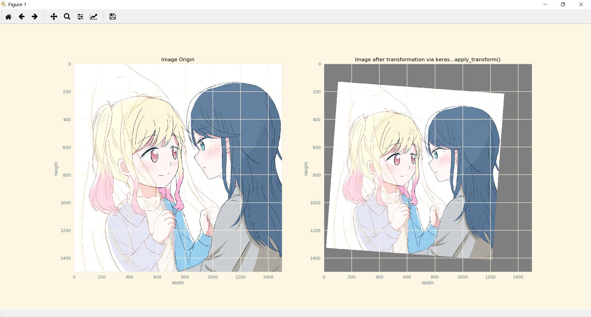
由此可见, keras.preprocessing.image.apply_transform更适合深度学习中进行图片的变换.

Attention!!

但是需要注意以下几点

这个函数只存在于Keras的1.0.2到2.1.6版本之间
由keras.preprocessing.image.load_img()导入图片得到的是一个PIL.JpegImagePlugin.JpegImageFile对象, 用keras.preprocessing.image.img_to_array()转换得到的是把RGB亮度映射到[0, 255]之间的张量, 但plt.imshow()接收的是[0, 1]之间的张量, 所以在使用plt.imshow()时, 如若需要传入的张量除以255, 使其亮度范围从[0, 255]映射至[0, 1];

References

¹. OpenCV: Open Source Computer Vision Library ↩

². 参考 qq_39507748的CSDN博客 opencv学习笔记三：使用cv2.GetAffineTransform()实现图像仿射, 同时也参考了其他文章 ⁸ ⁹ ¹⁰ ↩

³. 百度百科词条齐次坐标 ↩

⁴. 百度百科词条射影空间 ↩

⁵. 百度百科词条等价类 ↩

⁶. Robin Hartshorne, 代数几何, Springer, 1977 ↩

⁷. *Rocket_0911, “好久没发了….”, Lofter, 2022, post id: 1fcd09fb_2b46d3769 ↩

⁸. francislucien2017的CSDN博客 CV-Python核心操作: 图像属性/通道/位运算/色彩空间/缩放/阈值 ↩

⁹. xiaoniu-666的博客园文章 OpenCV之cv2.getAffineTransform+warpAffine ↩

¹⁰. qq_27261889的CSDN博客 python+opencv图像变换的两种方法cv2.warpAffine和cv2.warpPerspective ↩

¹¹. イットリウム^さん, “Under the Starlit Night”, Piapro, 2014, illustration id: fCH7 ↩

¹². Mathworks文档 Image Processing Toolbox ↩

¹³. Mathworks文档 imwarp ↩

¹⁴. Octave Forge - The image Package ↩

¹⁵. Missing Functions of the image Package ↩

¹⁶. 3434, “icsk部分集合”, Pixiv, 2021, artwork id: 95131145 ↩

QUST Data Science Research Association

青岛科技大学数据科学研究协会

数学建模实验 III 平面图形几何变换

Author: `sandyzikun`

Problem Description

Problem Analysis

Basic Methods

`OpenCV` Method `.resize`

`OpenCV` Method `.warpAffine`

Images in Linear Algebra

Modeling

Image Resizing

Image Shifting

Image Rotation

Affine Transformation

Processing Image with `OpenCV`

Solving

Extra

Attention!!

References

Problem Description

Problem Analysis

Basic Methods

OpenCV Method .resize

OpenCV Method .warpAffine

Images in Linear Algebra

Modeling

Image Resizing

Image Shifting

Image Rotation

Affine Transformation

Processing Image with OpenCV

Solving

Extra

Attention!!

References

`OpenCV` Method `.resize`

`OpenCV` Method `.warpAffine`

Processing Image with `OpenCV`